Difference Between read.csv and read_csv: A Practical Guide
Explore the differences between read.csv (base R) and read_csv (readr) for CSV import in R. Learn defaults, performance, typing, and best practices with practical guidance from MyDataTables.

In R, read.csv (base R) and read_csv (readr) serve the same purpose—importing comma-separated data—but they differ in defaults, data structures, performance, and ecosystem impact. Read_csv typically offers faster parsing, tibble output, and clearer type guessing, making it preferable for modern workflows; read.csv remains viable for legacy scripts and simpler, dependency-free use.
Overview: why the difference matters for data work
The primary difference between read.csv and read_csv centers on the library ecosystem and the resulting defaults and performance characteristics. For data analysts, developers, and business users evaluating CSV import routines, understanding how these two functions behave helps prevent subtle bugs and accelerates data pipelines. The keyword difference between read.csv and read_csv is central to this choice, especially as you integrate R into broader data workflows and reproducible analyses. MyDataTables emphasizes practical decisions over theoretical distinctions, so this guide balances foundational concepts with actionable guidance.
Defaults and behavior: what each function assumes by default
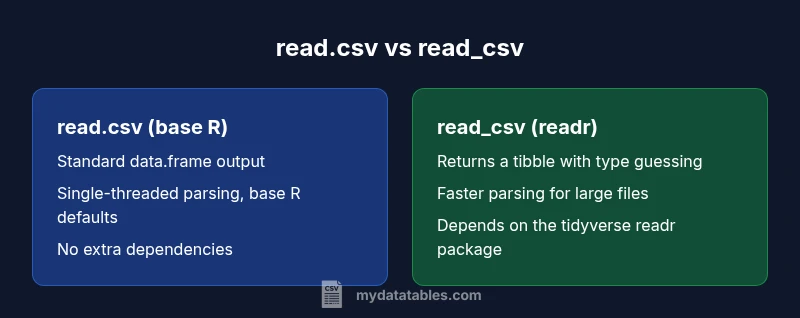
read.csv is part of base R. It default-handles a few behaviors that have evolved over time: a comma separator, a header row, and potential conversion of strings to factors depending on the R version. This legacy design makes read.csv familiar to early R users but can surprise newcomers when factors appear unexpectedly. read_csv, from the readr package in the tidyverse, normalizes many of these assumptions for modern workflows. It uses a comma delimiter by default, expects a header row, and returns a tibble rather than a base data.frame. For many teams, these defaults align more naturally with tidyverse pipelines and downstream tooling.
Performance and scalability: speed matters with large datasets
Performance matters when importing large CSV files. read_csv is optimized for speed through the tidyverse’s C-backed parsing backend, enabling faster reads on sizeable datasets. read.csv, while reliable, is generally slower on large inputs due to its base-R parsing mechanisms. If you routinely process multi-megabyte or gigabyte-scale CSV files, read_csv’s speed advantages translate into tangible time savings in ETL jobs and exploratory analyses. MyDataTables notes that performance differences compound as you run repeated imports within pipelines.
Typing, columns, and data shapes: what comes back to you
A key practical distinction is how each function infers and represents column types. read.csv returns a standard data.frame with columns typed according to its internal rules, and depending on the value of stringsAsFactors in your R version, text data may be converted to factors. read_csv returns a tibble with inferred column types, and readr exposes type information more explicitly, which can improve downstream data validation and transformation. This difference matters when you later wrap data in dplyr pipelines or join with other tibbles, as consistent types reduce the risk of implicit coercions.
Ecosystem and dependencies: building reproducible workstreams
read.csv is built into base R, requiring no extra packages. This makes it attractive for quick scripts and environments with minimal dependencies. read_csv requires the readr package (part of the tidyverse), which means adopting a broader ecosystem mindset and aligning with tidyverse conventions. If your project already relies on dplyr, ggplot2, and other tidyverse tools, read_csv integrates smoothly. For teams prioritizing minimal setup, read.csv remains a simple choice; for those pursuing modern, scalable pipelines, read_csv dovetails with a cohesive data science stack.
Compatibility across platforms and locale settings
CSV import can be sensitive to locale, encoding, and newline conventions. read_csv provides more explicit control and better handling of encoding and missing-value representations, which helps when moving data between platforms or languages. read.csv relies on base R defaults, which can be adequate in homogeneous environments but may require more manual adjustment when working with mixed locales or non-ASCII data. When portability is a priority, read_csv’s clearer options and consistent printing make cross-platform workflows more predictable.
Practical migration tips: moving from read.csv to read_csv (or not)
If you’re starting a new project, consider using read_csv to leverage tibble outputs and consistent type guessing, especially if you already work within the tidyverse. For legacy scripts, you can gradually migrate by wrapping read.csv calls in a conversion step like as_tibble(read.csv(...)) or by rewriting logic in tidyverse style. A pragmatic approach is to keep read.csv for one-off, quick analyses while updating longer-running ETL pipelines to read_csv for maintainability and performance. MyDataTables recommends incremental migration guided by your data team’s goals and constraints.
Common pitfalls and best practices: avoidable mistakes
Common mistakes include assuming default string handling will be identical across functions, underestimating the impact of factor conversion, and neglecting encoding issues in cross-team data sharing. Always verify the actual output type (data.frame vs tibble) and check column types after import. When using read_csv, explicitly specify col_types if you want to enforce or override automatic guessing. Document your data import choices so teammates understand the rationale and can replicate results.
Real-world usage patterns: when to pick which in practice
In practice, read.csv shines in quick, ad-hoc analyses or environments where adding dependencies is a barrier. read_csv dominates in reproducible research, data science projects, and production-style pipelines where speed, consistent types, and tidyverse integration matter. A pragmatic rule of thumb is: use read_csv for modern, scalable workflows and consider read.csv when working in legacy codebases or constrained environments where a minimal dependency footprint is essential.
Summary: balancing simplicity and modernity in CSV import
The difference between read.csv and read_csv is not simply about speed; it’s about ecosystem alignment, output structure, and predictability in data workflows. For teams investing in the tidyverse and scalable pipelines, read_csv offers a robust path forward. For those maintaining older scripts or teaching introductory examples, read.csv remains a reliable, dependency-light option. The MyDataTables approach is to evaluate context, then choose the function that best supports reproducible, performant analyses.
Comparison
| Feature | read.csv (base R) | read_csv (readr) |
|---|---|---|
| Defaults and separators | sep=',', header=TRUE; stringsAsFactors determined by R version | delim=',', col_names=TRUE; show_col_types=TRUE by default |
| Return type | data.frame (base R) | tibble (readr) |
| Performance on large files | slower parsing in many scenarios | faster due to optimized parsing |
| Type inference | base rules with stringsAsFactors depending on version | automatic type guessing with clear type information |
| Dependency footprint | no extra package needed (base) | requires readr (tidyverse) |
| Folder/printing behavior | standard data.frame printing | tibble printing with concise preview |
| NA handling | na.strings parameter exists; factors can appear | na handling exposed through readr options; clearer NA representation |
| Cross-language compatibility | typical for legacy scripts | better alignment with tidyverse data flows |
Pros
- read.csv is built into base R, no extra installation needed
- read_csv integrates with tidyverse, offering faster parsing for large files
- read_csv returns tibbles which are convenient in modern data pipelines
- read.csv has wide legacy compatibility across older scripts and tutorials
- read_csv provides clearer type information and warnings when parsing
Weaknesses
- read.csv may be slower on large datasets and can require extra factor handling
- read_csv adds a dependency on the tidyverse, which may not fit all projects
- tibbles from read_csv behave differently in printing and subsetting than data.frames
- Legacy read.csv scripts may be easier to understand for beginners familiar with base R
read_csv is generally preferred for modern, scalable data pipelines; read.csv remains viable for legacy code.
If you’re starting new work and value speed, explicit types, and tidyverse compatibility, choose read_csv. For legacy scripts or environments with minimal dependencies, read.csv stays a solid choice; plan gradual migration where feasible.
People Also Ask
What is the main difference between read.csv and read_csv?
The main difference is ecosystem and defaults: read.csv is base R and returns a data.frame with older default handling, while read_csv is from readr, returns a tibble with faster parsing and clearer type inference. This affects downstream processing in tidyverse workflows.
read.csv is base R and returns a data.frame, while read_csv is from readr and returns a tibble with faster parsing and clearer types.
Is read_csv faster than read.csv?
Generally, yes. read_csv uses a more optimized parsing engine in the tidyverse, which tends to perform better on larger CSV files. The exact speed gain depends on file size and system resources.
Yes, read_csv is typically faster for large CSVs due to optimized parsing.
Do I need to install the readr package to use read_csv?
Yes. read_csv is part of the readr package, which is in the tidyverse. If you’re not already using tidyverse, you’ll need to install and load readr to access read_csv.
Yes—read_csv comes from the readr package, so you need to install and load tidyverse to use it.
Can I use read.csv in a tidyverse workflow?
You can, but read_csv integrates more cleanly with tidyverse verbs like dplyr and ggplot2. In mixed codebases, you may convert read.csv results to tibbles using as_tibble.
Yes, you can use read.csv, but read_csv fits tidyverse workflows better.
How do I handle encoding issues when importing CSVs?
read_csv provides more explicit encoding control and better handling of non-ASCII data, while read.csv relies on base R locale settings. If encoding is important, specify encoding parameters or pre-process data accordingly.
read_csv offers clearer encoding control; with read.csv you depend on locale settings.
Which should beginners learn first, read.csv or read_csv?
For beginners, starting with read_csv in a tidyverse training path can be beneficial due to consistent type handling and modern workflows. If teaching legacy scripts, illustrate read.csv but note its limitations.
Begin with read_csv if you’re teaching modern data workflows; read.csv is fine for legacy examples.
Main Points
- Start with read_csv for new projects to align with tidyverse conventions
- Use read.csv for legacy codebases and minimal setups
- Expect data.frame vs tibble differences and adjust downstream code
- Prefer explicit col_types in read_csv when data types are uncertain
- Document your import strategy to improve reproducibility